ANOVA example

Example of One-Way Analysis of Variance

This is a quick introduction to one-way analysis of variance (ANOVA), taken from Moore and McCabe, Introduction to the Practice of Statistics, Freeman, New York, 1993. Let's begin with a clear statement of what ANOVA is used for:

Given "scores" from samples from several population groups, ANOVA is used to decide whether the differences in the samples' average scores are large enough to conclude that the groups' average scores are unequal. The null hypothesis is that all the groups have equal averages, and that any differences in the sample averages are due to chance. Then ANOVA computes a variable F on the basis of this hypothesis, and the larger the value of F, the more unlikely it is, and hence the more likely that at least one of the populations has an average different from the others. If F is not large enough, the conclusion is that all the populations have equal averages.

Moore and McCabe's discussion runs to some 50 pages; I have tried to summarize and supplement it in a mere 2 pages. Since the supplement involves some technical algebra, I have presented it in a separate document: Discussion in .pdf format. It includes some additional assumptions for ANOVA to be a valid test and describes Moore and McCabe's comments about the fulfilling of those assumptions.

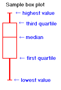
To describe what the variable F in ANOVA measures, we nearly copy a diagram from Moore and McCabe; but first, since it uses boxplots, a form of diagram not discussed in our text, we provide a sample:

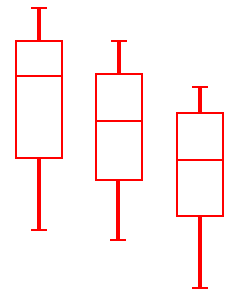Now if the group samples were distributed as shown in the box plots to the left, with large spreads about their centers, then small differences between the sample averages would be less noticeable, and less significant, than if the samples were distributed as shown on the right, with exactly the same group sample averages (or at least the same medians) but small spreads within samples.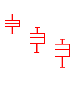

Thus, in order to see whether differences in sample averages from different groups are significant (i.e., if they indicate that the population groups from which the samples were drawn really have different averages), our computations must include measures of the spreads within the group samples. I.e., in deciding whether differences in sample averages are significant, we must also measure variation within the samples, of the data values from their respective sample averages, as well as measuring the spread of the sample averages from the grand average of all the data values. These spreads are related in formulas to yield a measure (the F mentioned above) of the spread of the different averages relative to the spreads within the samples. Here are the formulas; see the discussion linked above for more information:

Denote the number of groups by I, and use g as the variable running from 1 to I (the number of the group, just used as a label).
For each group g, denote by n_g the number of data values in the sample from that group. And denote by x_i,g the i-th data value in the sample from group g (as g runs from 1 to I and i runs from 1 to n_g).
Let N = n₁ + n₂ + ... + n_I, the total number of data values.
For each group g, denote by AV_g the average of the sample from group g, i.e., the sum of the x_i,g's (for that fixed g) divided by n_g.
Denote by AV the average of all the data values, i.e. the sum of all the x_i,g's divided by N (or, equivalently, the weighted average (n₁AV₁ + n₂AV₂ + ... + n_gAV_g)/N of the sample averages).
Denote by SSE the sum of the squares (x_i,g - AV_g)², as g runs from 1 to I and i runs from 1 to n_g. The initials stand for "sum of squared deviations due to error", but it would be better if we understood it as the sum of squared variations of values within the samples from their respective sample averages. [Remark: If we summed only the squares for a fixed g, divided by n_g, and took the square root, we would have the SD of the sample from group g. Since the square of the SD is called the "variance", we can begin to see where the term ANOVA comes from.]
Denote by SSG the sum of the squared differences (AV_g - AV)², where each term is repeated n_g times, according to the g in the subscript. The initials stand for "sum of squared deviations due to groups", i.e., the sum of the squared variations of the group averages from the overall average (with each squared variation repeated the right number of times to represent the size of that group). Note that there are the same total number of terms in finding SSE and SSG.
When we want to decide whether the sample averages from the different groups are significantly different from one another, there are DFE = N-I degrees of freedom in the choice of the individual data values, because we presume that the I sample averages are known; and the "mean squared variation due to error" is the quotient MSE = SSE/DFE.
And there are DFG=I-1 degrees of freedom in the choice of the sample average from each group, because the overall average is known (as are the sample sizes). The "mean squared variation due to groups" is MSG = SSG/DFG.
And finally denote by F the ratio MSG/MSE. Again, the bigger that F is, the more the variation between the group sample averages "dominates" the variation within the samples, and hence the less likely it is that the averages of the (whole) groups are really all (just about) equal, and that the differences in the averages of the samples from those groups were just chance.

Having computed the value of F, we can consult a table for the F-distribution to find the probability (p-value) of getting a value of F at least that large, given the two degrees of freedom (DFE and DFG) determined from the numbers of columns and entries in the table of data.

The formulas just described are obviously hard to follow, so let us "apply" them to the two sets of three box plots pictured earlier:

In both cases, I = 3.
We assume that the three samples used to make the box plots to the left contained the same numbers of data values as in the three samples to the right; i.e., the n₁'s, n₂'s and n₃'s were the same on the left and on the right -- but that the samples on the left displayed more variability within the samples than on the right.
So the sum N of the n_g's is the same for both.

(Look again at the two sets of box plots)

From the box plots, we see that the three sample medians on the left are respectively equal to those on the right; we hope (and assume) that means that the corresponding sample averages are also equal, i.e., that AV₁, AV₂ and AV₃ are the same on both sides.
Since the sample sizes n_g and the sample averages AV_g are the same on both sides, so are the overall averages AV.
Now comes the important part: The SSE is much larger on the left than on the right, because there is more variability within samples, while . . .
the SSG's are equal, since they depend only on sample averages AV_g, overall averages AV and sample sizes n_g.
The DFE's are equal, N - 3, and so the MSE is much larger on the left.
The DFG's are equal, 3 - 1 = 2, and so the MSG's are equal.
Thus, F = MSG/MSE is much larger on the right than on the left; so it should have a much smaller, i.e., more significant, p-value. Thus, with the samples on the right, we are more likely to reject the null hypothesis that the groups from which they were taken have equal averages.

Moore and McCabe's main example is an analysis of the table of data to the right. The caption reads as follows:

A study of reading comprehension in children compared three methods of instruction. As is common in such studies, several pretest variables were measured before any instruction was given. One purpose of the pretest was to see if the three groups of children were similar in their comprehension skills. One of the pretest variables was an "intruded sentences" measure, which measures one type of reading comprehension skill. The data for the 22 subjects in each group are given [to the right]. The three methods of instruction are called basal, DRTA and strategies. We use Basal, DRTA, and Strat as values for the categorical variable indicating which method each student received.

The point to note here is that the subjects are divided into three groups according to the method of instruction they will receive, but they haven't yet received any special instruction. Indeed, the point of the test is to see whether the abilities of the test groups are essentially equal before the instruction begins. The average of each column appears in red at the bottom. Obviously the averages in the three samples differ; the question is whether they differ significantly enough to make the test of reading comprehension methods worthless.

Theoretical nitpick

Basal	DRTA	Strat
4	7	11
6	7	7
9	12	4
12	10	7
16	16	7
15	15	6
14	9	11
12	8	14
12	13	13
8	12	9
13	7	12
9	6	13
12	8	4
12	9	13
12	9	6
10	8	12
8	9	6
12	13	11
11	10	14
8	8	8
7	8	5
9	10	8
10.5	9.7	9.1

Using the formulas above, we have:

I=3;
Numbering the Basal, DRTA and Strat groups as groups 1, 2 and 3 respectively, each one has 22 subjects in it, so n₁ = n₂ = n₃ = 22, and x_1,1 = 4, x_1,2 = 7, x_1,3 = 11, x_2,1 = 6, etc.;
N = 22 + 22 + 22 = 66;
AV₁ = 10.5, AV₂ = 9.7, AV₃ = 9.1 (at least approximately -- all figures except the degrees of freedom are approximate from here on);
AV = (22(10.5) + 22(9.7) + 22(9.1))/66 = 9.8;
SSE = (4 - 10.5)² + (7 - 9.7)² + (11 - 9.1)² + (6 - 10.5)² + . . . (a total of 66 terms) = 572.5;
SSG = 22(10.5 - 9.8)² + 22(9.7 - 9.8)² + 22(9.1 - 9.8)² = 20.6;
DFE = 66 - 3 = 63, and so MSE = 572.5/63 = 9.1;
DFG = 3 - 1 = 2, and so MSG = 20.6/2 = 10.3; and hence, finally,
F = 10.3/9.1 = 1.13.

And by consulting an F-distribution table with DFG = 2 and DFE = 63, we find that the probability of a F-value of at least 1.13 is about 33%, far too large for statistical significance. We conclude that the reading comprehension averages of the three groups of students are essentially identical before they receive their different forms of instruction.

But of course these formulas are evaluated, no longer by hand or even by calculator, but by computer. Indeed, the computer programs not only find the value of F but also find the associated p-value. Here is a screen shot from the Excel spreadsheet program, the result of using its built-in ANOVA Single Factor function on the data above. This function is available in the Tools menu under Data Analysis. (If you do not have Data Analysis in your Tools menu, see the first Excel help page linked to the course's index page.) It shows most of the values mentioned earlier and finally gives the value of F, about 3.14, that would have been large enough (given the two degrees of freedom) to conclude statistical significance (at the 5% level) of the differences between the group averages. Also, rather than the "error" vs. "groups" terminology, it uses the clearer "within groups" vs. "between groups".