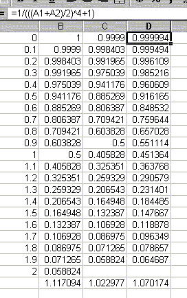
 These products were obtained by dividing
the interval of x-values from 0 to 2 into subintervals,
choosing an x-value in each of the subintervals,
evaluating the function
Several examples given in class
(on area under a curve, distance covered, and work done) turned
out to have the same numerical answer, given exactly by the
area of a region under a curve (and above the x-axis,
and between two vertical lines that determine the interval in
question), and approximated by a sum of products.
 These products were obtained by dividing
the interval of x-values from 0 to 2 into subintervals,
choosing an x-value in each of the subintervals,
evaluating the function
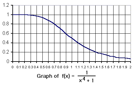 Here is a graph of
the function f. One thing to note is that it is
decreasing on the interval from 0 to 2, so that the maximum
f-value on each subinterval appears at the left endpoint
and the minimum at the right. The following graphics show how
to interpret the three sums of products above as sums of rectangular
areas related to this graph. Let's introduce the usual symbols
for this situation, at least as many as we can in HTML: The
major interval in question, here [0,2], is in general denoted
[a,b]. The points of division forming the subintervals,
here 0, 0.1, 0.2 and so on, are denoted x1,
x2, x3, and so on. So if there are
n subintervals (here there are 20), then there are
n+1 points of division (21 here), including the ends
x0=a and xn=b, and the i-th
point of division, counting from i=0, is xi.
The length of the i-th subinterval, from xi-1
to xi, is equal to
xi-xi-1; in this example, each is
equal to 0.1. It is usually denoted by a
capital delta, i.e., an equilateral triangle, in front of
xi, but a capital delta is not an HTML symbol,
so I can only write it as Delta xi. And finally,
the x-value chosen in the i-th subinterval from
xi-1 to xi as the point at
which the value of f will be found is denoted
x*i. It is the different choices for
x*i that give us the different approximations
in Columns B, C and D in the spreadsheet above.
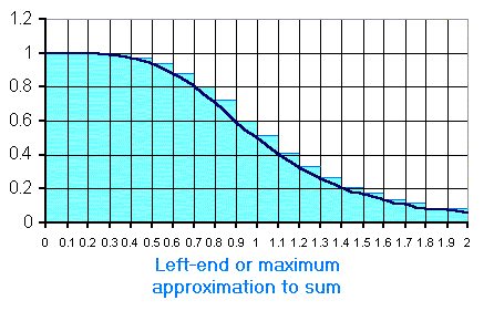 In this case the
points x*i chosen from the subintervals are
the left endpoints xi-1 of the subintervals,
which for this function are the points at which
the function takes on its maximum value. As a result, each of
the products is the area of a rectangle (in blue) that is at
least as tall as the function anywhere on that subinterval.
Therefore, the region under the curve is entirely covered by the
rectangles, with some small "triangle-like" pieces of the
rectangles extending above the curve. Thus, the approximation
of the area under the curve, 1.117094, given by this choice of
x*i's is an overestimate, by the sum of the
areas of those triangle-like pieces.
 In this case the
points x*i chosen from the subintervals are
the right endpoints xi of the subintervals,
which for this function are the points at which
the function takes on its minimum value. As a result, each of
the products is the area of a rectangle (in green) that is
never taller than the function throughout that subinterval.
Therefore, the rectangles are entirely covered by the
region under the curve, with some small "triangle-like" pieces of
the region under the curve that are not covered by the rectangles.
Thus, the approximation of the area under the curve, 1.022977,
given by this choice of x*i's is an
underestimate, by the sum of the areas of those triangle-like
pieces.
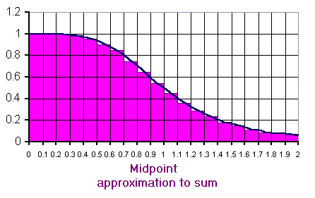 In this case the
points x*i chosen from the subintervals are
the midpoints (xi-1+xi)/2 of the
subintervals. As a result, each of
the products is the area of a rectangle (in purple) that is
below the curve at the left end and above it at the right.
Therefore, the total area of the triangles, 1.070174, is probably
a good approximation of the area under the curve: There are
some small "triangle-like" pieces of the region
under the curve that are not covered by the rectangles and
some small triangle-like pieces of the rectangles that are
not covered by the region under the curve, and so they are
likely to come close to cancelling each other out.