| from Group |
||
|---|---|---|
| #1: | 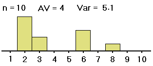 |
 |
| #2: | 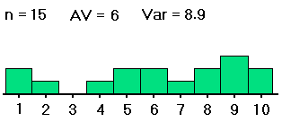 |
 |
| #3: | 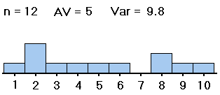 |
 |
This is a quick introduction to one-way analysis of variance (ANOVA). The "interludes" scattered along the way can be read after the reader has followed the main line of the argument. Let's begin with a clear statement of what ANOVA is used for:
Given "scores" from samples from several population groups, ANOVA is used to decide whether the differences in the samples' average scores are large enough to conclude that the groups' average scores are unequal. It is a significance test: it begins with the null hypothesis that all the groups have equal averages and that any differences in the sample averages are due to chance in, for example, the way the samples were taken. Then on the basis of this hypothesis, ANOVA computes the value of a variable F; the larger the value of F, the more unlikely it is to have occurred by chance, and hence the more likely that at least one of the populations has an average different from the others. If F is not large enough, the conclusion is that all the populations have equal averages.
Interlude One: The assumptions for ANOVA
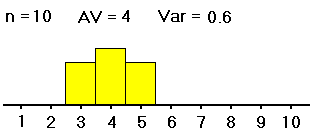
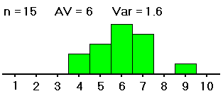
To describe what the variable F in ANOVA measures, let's consider two sets of samples from three groups.
| from Group |
||
|---|---|---|
| #1: | 2,2,2,2,3, 3,6,6,6,8 |
3,3,3,4,4, 4,4,5,5,5 |
| #2: | 1,1,2,4,5, 5,6,6,7,8, 8,9,9,9,10 |
4,4,5,5,5, 6,6,6,6,6, 7,7,7,7,9 |
| #3: | 1,2,2,2,3, 4,5,6,8,8, 9,10, |
3,3,4,4,5, 5,5,5,5,6, 7,8 |
| from Group |
||
|---|---|---|
| #1: |  |
 |
| #2: |  |
 |
| #3: |  |
 |
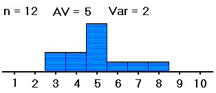
We want to know whether the averages of groups #1, #2 and #3 -- not the sample averages, which we have computed and are clearly all different, but the averages of the groups as a whole -- are all equal (probably about 5). If the samples were distributed as shown on the left (in both table and histogram), with large spreads about their averages, then small differences between the sample averages would be less noticeable, and less significant, than if the samples were distributed as shown on the right, with the same sample averages but small spreads within the samples. So with data as on the right, we would be more convinced that the group averages are different.
Thus, in order to see whether differences in averages of samples from different groups are significant (i.e., if they indicate that the population groups from which the samples were drawn really have different averages), our computations must include measures of the spreads within the group samples. That is, in deciding whether differences in sample averages are significant, we must also measure variation within the samples, of the data values from their respective sample averages, as well as measuring the spread of the sample averages from the grand average of all the data values. These spreads are related in formulas to yield a measure (the F mentioned above) of the spread of the different sample averages from the grand average versus the spreads within the samples. Here are the formulas:
Interlude Two: Notes on the formulas
Having computed the value of F, we can consult a table for the F-distribution to find the probability (p-value) of getting a value of F at least that large, given the two degrees of freedom (DFE and DFG) determined from the numbers of groups and data values.
Interlude Three: The F-distribution.
The formulas just described are obviously hard to follow, so let us apply them to the two sets of data mentioned earlier:
| from Group |
||
|---|---|---|
| #1: |  |
 |
| #2: |  |
 |
| #3: |  |
 |
But of course these formulas are evaluated, no longer by hand or even by calculator, but by computer. Indeed, the computer programs not only find the value of F but also find the associated p-value (on the basis of the two values of degrees of freedom), and often give the smallest value of F that would would be needed to yield statistical significance (the "critical F-value". Here are two screen shots from the Excel spreadsheet program, the result of using Excel's built-in ANOVA Single Factor function on the data above. This function is available in the Tools menu under Data Analysis. (If you do not have Data Analysis in your Tools menu, see the first Excel help page linked to our course's index page.) The screens show most of the values mentioned earlier. Also, rather than the "error" vs. "groups" terminology, it uses the clearer "within groups" vs. "between groups".
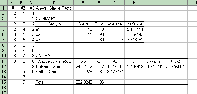 |
This screen shot shows the results of the data shown above on the left side, with large variations within the samples. |
| This one shows the results of the data above on the right, with small variations within the samples. Note that many of the values are the same, including "F crit". But the p-value on the right is much smaller; so with the data on the left we do not reject the null hypothesis that the group averages are different; while with the data on the right, we conclude that the averages of groups #1, #2 and #3 are different; the sample averages are not different merely by chance. |  |
Interlude Four: The Source of Variation Total