VFGEN § DDE

DDE_SOLVER

The DDE_SOLVER command creates Fortran 90 code that can be used with DDE_SOLVER_M, a Fortran 90 module created by S. Thompson and L. F. Shampine for solving differential delay equations.

The VFGEN DDE_SOLVER Command

A Fortran 90 file that can be used with the DDE_SOLVER_M module is created by the command

$ vfgen dde_solver vector_field_file.vf

The command will create the file [name].f90, where [name] is the name of the vector field defined in vector_field_file.vf.

The vector field must have at least one delay expression.

Options

demo

If the option demo=yes is given, the file [name]_demo.f90 is created. This program uses the default initial conditions and parameter values to generate a solution to the DDEs.
Default: demo=no

Example 1

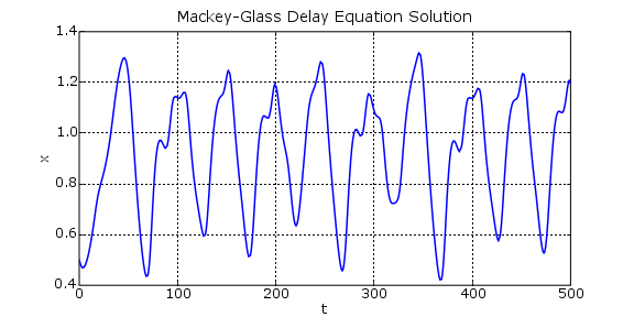
The Mackey-Glass equation is

x'(t) = -b*x + a*x(t-τ)/(1+x(t-τ)¹⁰)

Here is the Mackey-Glass vector field file: MackeyGlass.vf.
The files created by

$ vfgen dde_solver:demo=yes MackeyGlass.vf

are

To compile the demonstration program, I will use the gfortran compiler. (gfortran is easily installed in most Linux distributions. Another readily available Fortran compiler is g95. If you use g95, you may need to add the option -ffree-line-length-huge to the command; the lines generated by VFGEN often exceed 80 characters.)

First the DDE_SOLVER_M module must be downloaded and compiled. As of 29 April 2007, there is a .zip file on the DDE Solver web page. It contains two files: dde_solver_m.f90 and dde_solver_m_unix.f90. These files are identical except for the 'end-of-line' convention. I will use dde_solver_m_unix.f90.

To compile the solver module:

$ gfortran -c -w dde_solver_m_unix.f90

(I use the -w option because without it, gfortran prints many warnings about the code; as far as I can tell, the warnings do not actually cause any problems.)

To compile the demonstration program:

$ gfortran MackeyGlass.f90 MackeyGlass_demo.f90 dde_solver_m_unix.o -o MackeyGlass_demo

and to run it:

$ ./MackeyGlass_demo > mg.dat

Here is a plot of the data generated by MackeyGlass_demo, after the stoptime in MackeyGlass_demo.f90 was changed to 500:

Example 2

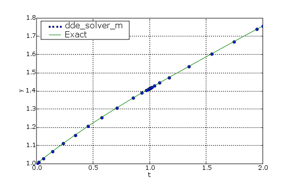
This example has a state-dependent delay. The DDE is

y'(t) = y(t)y(ln(y(t))-1)/(t+1)

y(t) = 1 t < 0
A vector field file for this system is sdd.vf. We create the Fortran 90 functions and demonstration program with the command

$ vfgen dde_solver:demo=yes sdd.vf

This creates the files

In Linux, we compile and run this program with the commands

$ gfortran sdd.f90 sdd_demo.f90 dde_solver_m_unix.o -o sdd_demo
$ ./sdd_demo > sdd.dat

Here is a plot of the result. The data computed by the DDE_SOLVER is plotted with blue dots; the exact solution is the green line.

For reference, the exact solution is
y(t) = t+1 for 0 ≤ t ≤ e-1
y(t) = exp((t+1)/e) for e-1 ≤ t ≤ exp(2)-1
y(t) = (e/(3-ln(t+1)))^e for exp(2)-1 ≤ t ≤ exp(3-exp(1-e))-1

The example was taken from "DKLAG6: A Code Based on Continuously Imbedded Sixth Order Runge-Kutta Methods for the Solution of State Dependent Functional Differential Equations", by S. P. Corwin, D. Sarafyan, and S. Thompson, and they give their source of the equation as "Developing a Delay Differential Equation Solver" by C. A. H. Paul (J. Appl. Num. Math., Vol. 9, pp. 403-414, 1992).

Example 3

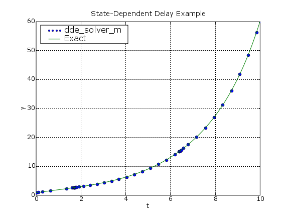
This is another example with a state-dependent delay. The DDE is

y'(t) = (1/2)(t+1)^(-1/2)y(y-sqrt(2))

y(t) = 1 t < 0
A vector field file for this system is sddfn.vf. We create the Fortran 90 functions and demonstration program with the command

$ vfgen dde_solver:demo=yes sddfn.vf

This creates the files

In Linux, we compile and run this program with the commands

$ gfortran sddfn.f90 sddfn_demo.f90 dde_solver_m_unix.o -o sddfn_demo
$ ./sddfn_demo > sdd.dat

Here is a plot of the result, after changing the variables in the demo program to relerr=1D-9, abserr=1D-11, and stoptime=2.0. The data computed by the DDE_SOLVER is plotted with blue dots; the exact solution is the green line.

For reference, the exact solution is
y(t) = (t+1)^(1/2) for 0 ≤ t ≤ 1
y(t) = (t+1)/4 + 1/2 + (1-sqrt(2)/2)(t+1)^(1/2) for 1 ≤ t ≤ 2

The example was taken from "High Order Methods for State-Dependent Delay Differential Equations with Nonsmooth Solutions", by A. Feldstein and K. W. Neves (SIAM J. Numer. Anal., Vol. 21, No. 5., pp. 844-863, October, 1984).