VFGEN § Delay2ODE

Delay2ODE

A delay can be approximated by using a finite-dimensional system of differential equations. This command provides the ability to automatically generate such an approximation from a differential delay equation.

The delay2ode command generates a new vector field file from an existing file that contains delays. The new vector field will be a system of ordinary differential equations in which the delays have been replaced by finite dimensional approximations.

Background. Suppose

y(t) = x(t-δ) Then, of course, y(t+δ) = x(t) Let N > 0 be an integer. We can write the previous equation as

y₁(t + δ/N) = x(t)

y₂(t + δ/N) = y₁(t)

.

.

.

y_N(t + δ/N) = y_N-1(t)

and y_N(t) = y(t). We expand y_k(t+δ/N) in a Taylor series, and then approximate the system by keeping only terms up to order p in the series. We obtain a differential equation of order p for each y_k. When p > 1, we convert the differential equation into a system of p equations. We write the variables in the k^th system as y_1,k, y_2,k, ..., y_p,k. Then y_k = y_1,k.

When p=1, we obtain

y_k' = (N/δ)(y_k-1 - y_k) (The case p=1 is equivalent to assuming that the delay time is a random variable whose probability distribution function is an Erlang distribution with shape parameter N.)

When p=2, we obtain

y_1,k' = y_2,k

y_2,k' = (2N/δ)(-y_2,k + (N/δ)(y_1,k-1 - y_1,k))

When p=3, we obtain

y_1,k' = y_2,k

y_2,k' = y_3,k

y_3,k' = (3N/δ) (-y_3,k - (2N/δ)(y_2,k - (N/δ)(y_1,k-1 - y_1,k)))

(p=4 has not yet been implemented. For p > 4, the linear system is unstable.)

Options

p	Order of the approximation. As explained above, this is the order of the Taylor series retained in the approximation of a ``small'' delay. Only p=1, p=2, and p=3 are allowed. Default: p=1
N	Number of grid points in the approximation to the delayed expression in the delay interval. Default: N=10

Bugs

VFGEN versions 2.0.0 and 2.1.0 will crash ("Segmentation fault" in Linux) if the second argument to a delay function is not a single symbol. For example, suppose tau and b are Parameters. Then delay(x,tau) is fine, but delay(x,1) and delay(x,b*tau) will cause VFGEN to crash. I hope to fix this in 2.1.1. In the mean time, if you want to try the delay2ode command, always use a single symbol (either a Constant, a Parameter, or an Expression) as the second argument of the delay function.

Example 1

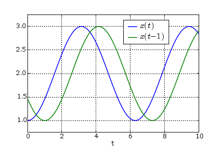
We consider the equation

x'(t) = sin(t), x(0)=1 Of course, this is not a delay equation. In fact, it is a trivial differential equation; we can simply integrate to obtain x(t) = -cos(t) + 2

We create a delayed copy of x(t) by defining an expression with the formula delay(x,h) Here is the vector field file simpledelay.vf. We create a new vector field with the command

$ vfgen delay2ode:N=12,p=2 simpledelay.vf > simpledelay_2ode.vf

Note that, unlike most VFGEN commands, the ouput is sent to the console rather than a file. In this example, we have redirected the output to the file simpledelay_2ode.vf. The name of the new vector field will be the name of the old vector field with "_2ode" appended to it.

We can now apply VFGEN to this new vector field to create a solver. The following commands create and compile a solver written in C that uses the GSL library. (See the GSL section for more information about using the GSL command of VFGEN.)

$ vfgen gsl:demo=yes simpledelay_2ode.vf
$ make -f Makefile-simpledelay_2ode

Then the command

$ ./simpledelay_2ode_demo relerr=1e-12 > outp2n12.dat

runs the solver, and writes the solution to the file outp2n12.dat. (Setting relerr=1e-12 is a bit of a "hack" to force the solver to generate reasonably dense output.) This file has 26 columns of data. The first two columns are t and x(t). The remaining 24 columns are the variables generated by VFGEN to approximate the delay. In particular, column 25 contains the approximation of x(t-h). Here is a plot of x(t) and x(t-h) from the data file. (The delay is h=1.)

Example 2: The Mackey-Glass Equation

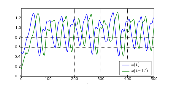
The Mackey-Glass equation is

x'(t) = -b*x + a*x(t-τ)/(1+x(t-τ)¹⁰)
A vector field file for this system is MackeyGlass.vf.

We create a new vector field with the command

$ vfgen delay2ode:N=25,p=3 MackeyGlass.vf > MackeyGlass_2ode.vf

(I have chosen to break up the delay interval into 25 subintervals, and use a third order approximation for each subinterval.) This creates the files MackeyGlass_2ode.vf.

The following commands create and compile a solver for this approximation to the delay equation.

$ vfgen gsl:demo=yes MackeyGlass_2ode.vf
$ make -f Makefile-MackeyGlass_2ode

The following command runs the solver:

$ ./MackeyGlass_2ode_demo relerr=1e-8 abserr=1e-10 stoptime=500 > mg.dat

This plot shows the solution x(t), along with the (approximate) delayed expression x(t-17):

(Another example in which the delay2ode command is used to approximate the Mackey-Glass equation with a finite dimensional system is given in the VFGEN auto command documentation.)